# Download and install SIPNET v1.3.0
source(
here::here(
"documentation/tutorials/Demo_1_Basic_Run/download_sipnet.R"
)
)Uncertainty Analysis Using PEcAn
1 Introduction
In Demo 2 we will be looking at how PEcAn can use information about parameter uncertainty to perform three automated analyses:
- Ensemble Analysis: Repeat numerous model runs, each sampling from the parameter uncertainty, to generate a probability distribution of model projections. Allows us to put a confidence interval on the model. Demo 1 shows this in action.
- Sensitivity Analysis: Repeats numerous model runs to assess how changes in model parameters will affect model outputs. Allows us to identify which parameters the model is most sensitive to.
- Uncertainty Analysis: Combines information about model sensitivity with information about parameter uncertainty to determine the contribution of each model parameter to the uncertainty in model outputs. Allow us to identify which parameters are driving model uncertainty.
This demo shows how to run an uncertainty analysis workflow in PEcAn using an R-based Quarto notebook. It covers loading settings, configuring models, running simulations, and performing sensitivity analyses to assess uncertainty and parameter importance. This programmatic approach complements the web-based PEcAn interface.
Context & modeling scenario:
We simulate plant and ecosystem carbon balance (Net Primary Productivity and Net Ecosystem Exchange) at the AmeriFlux Niwot Ridge Forest site (US‑NR1) during the year 2004. We use SIPNET parameterized as a temperate conifer PFT and driven by AmeriFlux meteorology following the analysis in Moore et al. (2007). This notebook also provides a compact template that can be extended to more years, locations, and PFTs.
What this notebook does:
- Configure a PEcAn workflow by loading and validating a
pecan.xmlsettings file. - Run a set of ecosystem model simulations by writing model configuration files and then running SIPNET.
- Quantify uncertainty using sensitivity analyses, and variance decomposition.
- Visualize results to identify important parameters and how they influence model variance.
- Change configuration settings and re-run the workflow.
1.1 Prerequisites
To run this notebook, you will need to install PEcAn and its dependencies, as well as download the SIPNET model binary.
1.1.1 PEcAn packages and dependencies.
# Enable repository from pecanproject
options(repos = c(
  pecanproject = 'https://pecanproject.r-universe.dev',
  CRAN = 'https://cloud.r-project.org'))
install.packages(c('PEcAn.all', 'PEcAn.SIPNET'))
A valid pecan.xml configuration file. Start with the example at pecan/documentation/tutorials/Demo_02_Uncertainty_Analysis/pecan.xml.
1.1.2 SIPNET v1.3.0
If you haven’t already installed the SIPNET model, you can do so by running the following code. This will download the SIPNET binary to demo_outdir/sipnet and make it executable.
Note: The
demo_outdirdirectory will be created inside of your PEcAn installation, atdocumentation/tutorials/Demo_02_Uncertainty_Analysis/demo_outdir/. This directory will contain the SIPNET binary as well as the output generated by PEcAn in this demo.
Note: You can find the most recent version of the SIPNET binary at: SIPNET GitHub Releases, but this notebook is designed to work with SIPNET v1.3.0.
2 Load PEcAn Packages
First, we need to load the PEcAn R packages. These packages provide all the functions we’ll use to run the workflow.
# Load the PEcAn.all package, which includes all necessary PEcAn functionality
library("PEcAn.all")
Loading required package: PEcAn.DBLoading required package: PEcAn.settingsLoading required package: PEcAn.MALoading required package: PEcAn.loggerLoading required package: PEcAn.utilsLoading required package: PEcAn.uncertaintyLoading required package: PEcAn.data.atmosphereLoading required package: PEcAn.data.landLoading required package: PEcAn.data.remoteLoading required package: PEcAn.assim.batchLoading required package: PEcAn.emulatorLoading required package: PEcAn.priorsLoading required package: PEcAn.benchmarkLoading required package: PEcAn.remoteLoading required package: PEcAn.workflowset.seed(20260325)3 Load PEcAn Settings File
Use the XML settings file (pecan.xml) exactly as in the Demo 1 Basic Run tutorial. See the “Load PEcAn Settings File” section of Demo 1 for a more detailed walkthrough of fields and schema. In this tutorial we focus on settings relevant to this notebook and explain the additional options associated with uncertainty analysis.
3.1 Settings
Example settings for this demo live at pecan/documentation/tutorials/Demo_02_Uncertainty_Analysis/pecan.xml and you can read more about the settings in the PEcAn Documentation, and section focused on sensitivity analysis settings in particular.
There is no <ensemble> block in this file. A sensitivity analysis and an ensemble are separate runs, each with its own settings and its own design, so this demo carries only the sensitivity analysis and Demo 1 covers the ensemble.
Open that settings file and look at the sensitivity analysis section. You can modify these settings to change the variable being analysed and the quantiles each parameter is moved to. Some of the key settings in this demo include:
Output variable
The output variable for the sensitivity analysis is set to NPP (Net Primary Productivity). You can change this to other variables like NEE (Net Ecosystem Exchange), LAI (Leaf Area Index), ET (Evapotranspiration), etc. You can also specify multiple variables by providing a vector of variable names (e.g., c("NPP", "NEE", "LAI")) to analyze uncertainty across several ecosystem processes simultaneously.
Sensitivity analysis quantiles
PEcAn’s sensitivity analysis includes a handy shortcut that converts a specified standard deviation into its normal quantile equivalent. In the example pecan.xml, these are set to -1, 1 (the median value, 0, occurs by default) which are converted internally to the 15.9th and 84.1th quantiles of the parameter distribution. You can add more quantiles to explore a wider range of parameter values: {-3, -2, -1, 1, 2, 3} is often used in practice.
By working in quantiles relative to each parameter’s distribution, the sensitivity and variance decomposition reflect sensitivity across the range of parameter values. Many sensitivity analyses tools use a fixed perturbation size such as the mean +/- 10%. PEcAn’s SA does not take this approach because it does not capture the uncertainty across the parameter distribution and can not be used for variance decomposition.
3.2 Load the settings file
settings_path <- here::here("documentation/tutorials/Demo_02_Uncertainty_Analysis/pecan.xml")

settings <- PEcAn.settings::read.settings(settings_path)

settings <- PEcAn.settings::prepare.settings(settings)
See Demo 1 Section 6 for details on what these functions do. Briefly, they read the XML file, convert it into an R list object that PEcAn can use, check that settings are valid, fill in defaults, and create the output directory.
4 Write Model Configuration Files
This step decides which model runs to do, then writes the configuration files for them.
generate_OAT_SA_design() builds the sensitivity analysis design: one row per run. The first run holds every parameter at its median, and each run after that moves a single trait to one of its quantiles while everything else stays at the median. That is what makes the effect of each parameter separable. It returns the parameter samples alongside the design, since the design’s indices only mean anything together with the samples they point into.
runModule.run.write.configs() then takes that whole object and writes the SIPNET configuration files.
design <- PEcAn.uncertainty::generate_OAT_SA_design(settings)

settings <- PEcAn.workflow::runModule.run.write.configs(
  settings,
  input_design = design
)
Loading required package: PEcAn.SIPNETThe design carries labels saying what each run is, so it goes to the sensitivity runs without anything having to inspect the settings. An ensemble is a separate call with its own design, which is what Demo 1 does.
You can call runModule.run.write.configs() without a design and it will build one itself, but that path is deprecated and will warn. Building it yourself also lets you look at it first: design$design_matrix is the table of runs, and design$samples holds the parameter draws behind it.
5 Run Model Simulations
This section executes the SIPNET simulations and retrieves the results.
It uses the function runModule_start_model_runs(settings) to initiate the model runs using the configuration files generated in the previous step.
PEcAn.workflow::runModule_start_model_runs(settings)
  |
  |                                                                      |   0%
  |
  |==                                                                    |   3%
  |
  |====                                                                  |   5%
  |
  |=====                                                                 |   8%
  |
  |=======                                                               |  10%
  |
  |=========                                                             |  13%
  |
  |===========                                                           |  15%
  |
  |=============                                                         |  18%
  |
  |==============                                                        |  21%
  |
  |================                                                      |  23%
  |
  |==================                                                    |  26%
  |
  |====================                                                  |  28%
  |
  |======================                                                |  31%
  |
  |=======================                                               |  33%
  |
  |=========================                                             |  36%
  |
  |===========================                                           |  38%
  |
  |=============================                                         |  41%
  |
  |===============================                                       |  44%
  |
  |================================                                      |  46%
  |
  |==================================                                    |  49%
  |
  |====================================                                  |  51%
  |
  |======================================                                |  54%
  |
  |=======================================                               |  56%
  |
  |=========================================                             |  59%
  |
  |===========================================                           |  62%
  |
  |=============================================                         |  64%
  |
  |===============================================                       |  67%
  |
  |================================================                      |  69%
  |
  |==================================================                    |  72%
  |
  |====================================================                  |  74%
  |
  |======================================================                |  77%
  |
  |========================================================              |  79%
  |
  |=========================================================             |  82%
  |
  |===========================================================           |  85%
  |
  |=============================================================         |  87%
  |
  |===============================================================       |  90%
  |
  |=================================================================     |  92%
  |
  |==================================================================    |  95%
  |
  |====================================================================  |  97%
  |
  |======================================================================| 100%
The PEcAn workflow will take a longer time to complete than in Demo 1 because we have just asked for over a hundred model runs. Once the runs are complete we will continue.
6 Fetch Model Outputs
Next we convert all of the model output from the previous run to a standard format that PEcAn can use for analysis. This is done using the runModule.get.results() function.
runModule.get.results(settings)7 Sensitivity Analysis
Next, we use the outputs from the previous step to perform sensitivity analyses.
Sensitivity Analysis: Systematically varies individual parameters to assess their influence on model outputs. This identifies which parameters most strongly affect model predictions and helps prioritize parameter refinement efforts.
runModule.run.sensitivity.analysis(settings)$coef.vars
growth_resp_factor leaf_turnover_rate
0.52374704 0.87942430
root_respiration_rate root_turnover_rate
0.57746880 0.57076842
Amax leaf_respiration_rate_m2
0.56971262 0.55674422
SLA leafC
0.77640702 0.02629420
Vm_low_temp AmaxFrac
0.01097839 0.11569334
psnTOpt stem_respiration_rate
0.03403173 0.57964461
extinction_coefficient half_saturation_PAR
0.13866293 0.43006586
dVPDSlope dVpdExp
0.53581232 0.28716913
veg_respiration_Q10 fine_root_respiration_Q10
0.17313621 0.32208893
coarse_root_respiration_Q10
0.32648810
$elasticities
growth_resp_factor leaf_turnover_rate
0.00000000 0.02568241
root_respiration_rate root_turnover_rate
-0.02575450 0.05356806
Amax leaf_respiration_rate_m2
2.76097469 -2.03578673
SLA leafC
0.70748382 0.13727194
Vm_low_temp AmaxFrac
1.01801934 2.39620082
psnTOpt stem_respiration_rate
1.01060446 -1.45093209
extinction_coefficient half_saturation_PAR
-0.57357264 -1.25301797
dVPDSlope dVpdExp
-0.17135558 0.09486454
veg_respiration_Q10 fine_root_respiration_Q10
6.26873860 0.08528698
coarse_root_respiration_Q10
-0.20787552
$sensitivities
growth_resp_factor leaf_turnover_rate
0.000000e+00 1.130463e-10
root_respiration_rate root_turnover_rate
-2.489888e-12 5.156632e-11
Amax leaf_respiration_rate_m2
6.597067e-10 -1.970054e-09
SLA leafC
2.479184e-10 1.313050e-11
Vm_low_temp AmaxFrac
-9.956498e-10 1.546741e-08
psnTOpt stem_respiration_rate
2.489396e-10 -1.409878e-10
extinction_coefficient half_saturation_PAR
-5.548284e-09 -3.911165e-10
dVPDSlope dVpdExp
-6.393206e-09 2.293504e-10
veg_respiration_Q10 fine_root_respiration_Q10
1.516052e-08 1.282404e-10
coarse_root_respiration_Q10
-3.149514e-10
$variances
growth_resp_factor leaf_turnover_rate
2.117791e-50 2.448863e-20
root_respiration_rate root_turnover_rate
5.179353e-21 2.477726e-20
Amax leaf_respiration_rate_m2
6.038184e-17 2.882181e-17
SLA leafC
1.077233e-17 8.188934e-22
Vm_low_temp AmaxFrac
8.912733e-18 1.801301e-18
psnTOpt stem_respiration_rate
6.275273e-18 1.658119e-17
extinction_coefficient half_saturation_PAR
1.481172e-19 6.842910e-18
dVPDSlope dVpdExp
1.995797e-19 1.770854e-20
veg_respiration_Q10 fine_root_respiration_Q10
2.808673e-17 1.980436e-20
coarse_root_respiration_Q10
1.078595e-19
$partial.variances
growth_resp_factor leaf_turnover_rate
1.252949e-34 1.448822e-04
root_respiration_rate root_turnover_rate
3.064263e-05 1.465898e-04
Amax leaf_respiration_rate_m2
3.572373e-01 1.705186e-01
SLA leafC
6.373237e-02 4.844823e-06
Vm_low_temp AmaxFrac
5.273044e-02 1.065704e-02
psnTOpt stem_respiration_rate
3.712642e-02 9.809936e-02
extinction_coefficient half_saturation_PAR
8.763063e-04 4.048474e-02
dVPDSlope dVpdExp
1.180774e-03 1.047691e-04
veg_respiration_Q10 fine_root_respiration_Q10
1.661696e-01 1.171686e-04
coarse_root_respiration_Q10
6.381295e-04
growth_resp_factor leaf_turnover_rate root_respiration_rate
15.866 4.838975e-09 4.540769e-09 4.923092e-09
50 4.838975e-09 4.838975e-09 4.838975e-09
84.134 4.838975e-09 4.881666e-09 4.752644e-09
root_turnover_rate Amax leaf_respiration_rate_m2 SLA
15.866 4.551520e-09 -7.292932e-09 1.016052e-08 9.474297e-10
50 4.838975e-09 4.838975e-09 4.838975e-09 4.838975e-09
84.134 4.902221e-09 1.071740e-08 -6.773679e-10 5.616272e-10
leafC Vm_low_temp AmaxFrac psnTOpt
15.866 4.793754e-09 7.056707e-09 3.127530e-09 -4.998039e-09
50 4.838975e-09 4.838975e-09 4.838975e-09 4.838975e-09
84.134 4.844983e-09 1.853749e-09 6.297118e-09 7.814714e-09
stem_respiration_rate extinction_coefficient half_saturation_PAR
15.866 9.972994e-09 5.294348e-09 8.338709e-09
50 4.838975e-09 4.838975e-09 4.838975e-09
84.134 3.522819e-10 4.383285e-09 2.180100e-09
dVPDSlope dVpdExp veg_respiration_Q10 fine_root_respiration_Q10
15.866 5.271896e-09 4.646390e-09 -2.839443e-09 4.587255e-09
50 4.838975e-09 4.838975e-09 4.838975e-09 4.838975e-09
84.134 4.217896e-09 4.958194e-09 9.593516e-09 4.903486e-09
coarse_root_respiration_Q10
15.866 5.221299e-09
50 4.838975e-09
84.134 4.447164e-098 PEcAn Outputs
8.1 Output Directory Structure
These are the key folders and files that will be created under the directory defined by settings$outdir (e.g., demo_outdir in the example). The file contents are described in the next section.
We discussed the output directory in Demo 1 (Basic Run), but now there are additional outputs from the sensitivity and variance decomposition analyses.
demo_outdir/
├── run/                                    # Configuration & execution metadata
│   ├── runs.txt                           # List of run IDs
│   └── SA-*-*/                           # Sensitivity analysis run directories
├── out/                                   # Raw model outputs by run ID
│   └── <runid>/                          # E.g., daily or sub-daily SIPNET output files
├── samples.Rdata                         # Parameter samples used for the SA runs
├── sensitivity.output.*.Rdata            # SA model outputs
├── sensitivity.results.*.Rdata           # Processed SA results
├── sensitivity.samples.*.Rdata           # SA parameter samples
├── variance.decomposition.*.pdf          # Variance decomposition analysis
├── pft/                                  # Parameter (prior/posterior) files per PFT
│   └── temperate.coniferous/
└── sipnet                                # SIPNET binary (downloaded earlier)
8.1.1 Model outputs and logs
- Standardized netCDF files (
[year].nc) for analysis and visualization - Raw model output (for SIPNET, e.g.,
sipnet.outper run) logfile.txtwith model and workflow messages- Note:
pft/contains parameter files used in estimation; see the parameter-estimation tutorial (Demo 3) for details
9 Understanding PEcAn Uncertainty Analysis Outputs
After running the sensitivity analysis, PEcAn generates several important outputs that help you understand model uncertainty and parameter sensitivity.
The samples.Rdata file contains the parameter values used in the sensitivity analysis runs, in an object called sa.samples.
9.1 Sensitivity Analysis Outputs
The sensitivity analysis generates:
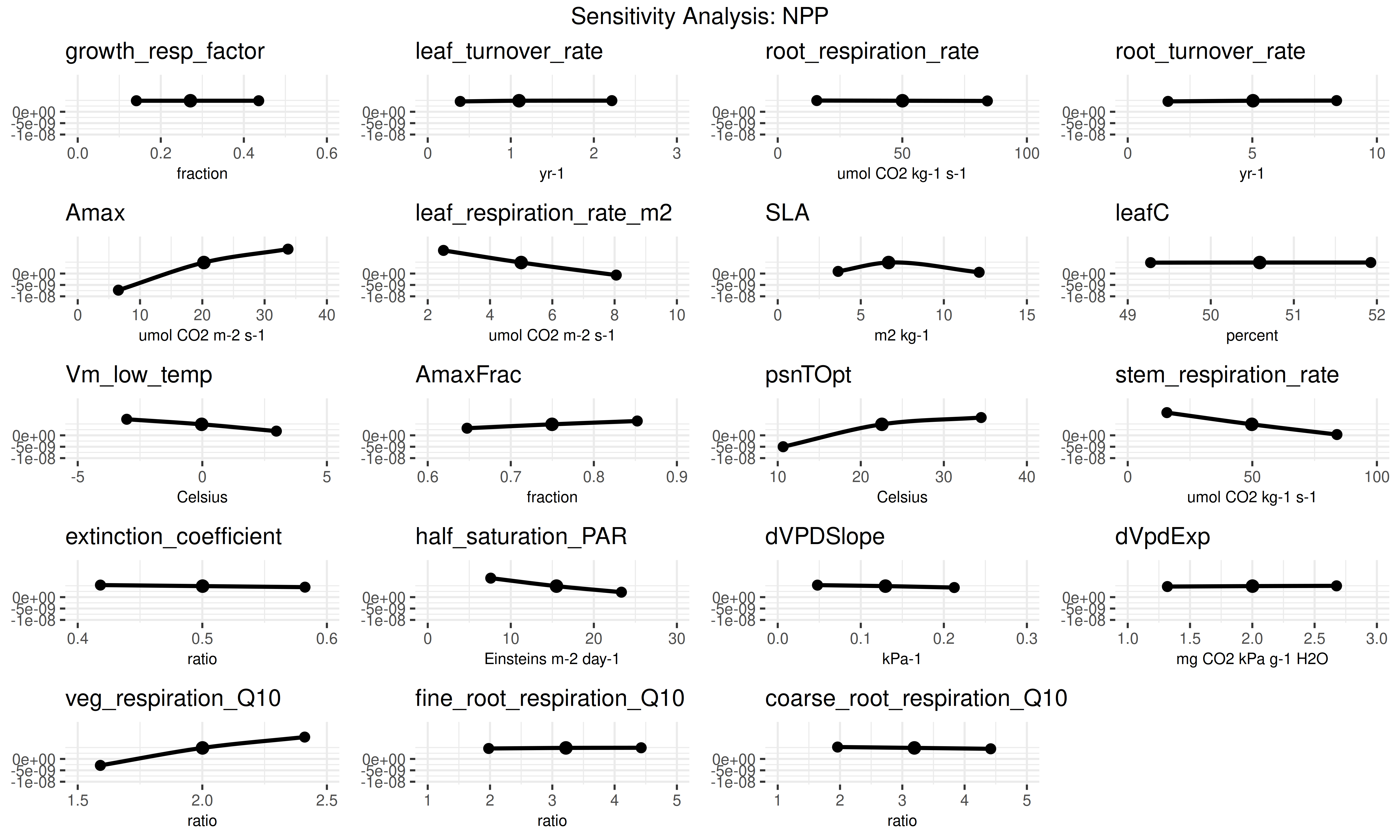
sensitivity.analysis.[RunID].[Variable].[StartYear].[EndYear].pdf: Raw data points from univariate analyses with spline fits.sensitivity.output.[RunID].[Variable].[StartYear].[EndYear].Rdata: Model outputs corresponding to parameter variations.sensitivity.analysis.[RunID].[Variable].[StartYear].[EndYear].pdfshows the raw data points from univariate one-at-a-time analyses and spline fits through the points. Open this file to determine which parameters are most and least sensitive.
9.2 Variance Decomposition Outputs
The variance decomposition produces:
variance.decomposition.[RunID].[Variable].[StartYear].[EndYear].pdf: Three-column analysis showing:- Coefficient of variation (normalized posterior variance)
- Elasticity (normalized sensitivity)
- Partial standard deviation of each parameter
9.3 Interpreting the Results
Variance Decomposition Analysis:
- Parameters are sorted by their contribution to model output uncertainty (the right column).
- Identify parameters that are:
- Highly sensitive but low uncertainty.
- Highly uncertain but low sensitivity.
- Both sensitive and uncertain.
- Identify parameters that are both sensitive and uncertain for future constraint with data or expert knowledge.
- Potential gotchas:
- Flat sensitivity curves: check that parameter values were correctly generated and read by the model.
- Parameters with high uncertainty: consider revising priors.
- Multi-modal or otherwise unexpected parameter distributions: check that parameter was specified correctly.
Choose the parameter that you think provides the most efficient means of reducing model uncertainty and propose how you might best reduce uncertainty in this process. In making this choice remember that not all processes in models can be directly observed, and that the cost-per-sample for different measurements can vary tremendously (and thus the parameter you measure next is not always the one contributing the most to model variability). Also consider the role of parameter uncertainty versus model sensitivity in justifying your choice of what parameters to constrain.
10 Visualize Uncertainty Analysis Results
This section loads the results from the uncertainty analyses and generates plots directly in the notebook. This provides an immediate view of the sensitivity plots and variance decomposition.
10.1 Sensitivity and Variance Decomposition Visualization
This block visualizes the results of the sensitivity analysis. The plots show how sensitive the model output is to changes in each parameter and which parameters contribute most to the overall uncertainty.
# --- 1. Define Helper Variables ---
# Extract key variables from the settings object to simplify file path construction
# and plotting. This makes the code cleaner and easier to read.
variable <- settings$sensitivity.analysis$variable
pft <- settings$pfts[[1]]
start.year <- lubridate::year(settings$run$start.date)
end.year <- lubridate::year(settings$run$end.date)

# --- 2. Load Sensitivity Analysis Results ---
vars <- settings$sensitivity.analysis[names(settings$sensitivity.analysis) == "variable"]
variables <- unlist(vars)

for (var in variables) {
  # Construct the path to the sensitivity analysis results file
  sens_file <- PEcAn.uncertainty::sensitivity.filename(
    settings,
    prefix = "sensitivity.results",
    all.var.yr = FALSE
  )

  if (file.exists(sens_file)) {
    PEcAn.logger::logger.info(paste("Plotting sensitivity results for variable:", var, "from", basename(sens_file)))

    sens_env <- new.env()
    load(sens_file, envir = sens_env)
    sensitivity.results <- sens_env$sensitivity.results

    # --- 3. Generate Sensitivity Plots ---
    if (!is.null(sensitivity.results[[pft$name]]$sensitivity.output)) {
      sa_plots <- PEcAn.uncertainty::plot_sensitivities(
        sensitivity.results[[pft$name]]$sensitivity.output
      )
      # Explicitly print the plot
      gridExtra::grid.arrange(
        grobs = sa_plots, ncol = floor(sqrt(length(sa_plots))),
        top = paste("Sensitivity Analysis:", var)
      )
    }

    # --- 4. Generate Variance Decomposition Plots ---
    if (!is.null(sensitivity.results[[pft$name]]$variance.decomposition.output)) {
      vd_plots <- PEcAn.uncertainty::plot_variance_decomposition(
        sensitivity.results[[pft$name]]$variance.decomposition.output
      )
      # Explicitly print the plot
      vd_plots + ggplot2::ggtitle(paste("Variance Decomposition:", var))
    }
  } else {
    PEcAn.logger::logger.warn(paste("Could not find sensitivity results file for variable:", var))
  }
}
11 Customizing Sensitivity Analysis Parameters (Optional)
11.1 (Optional) Use this section only if you want to override the default sensitivity analysis parameters. Skip if defaults are sufficient.
Important: If you modify the sensitivity analysis parameters in this section, re-run Section Section 7 and then Section Section 10 to regenerate outputs and plots.
# Set the quantiles (in standard deviations) for parameter distribution in sensitivity analysis
settings$sensitivity.analysis$quantiles$sigma <- c(-2, -1, 1, 2)

# Specify the variable to be analyzed in sensitivity analysis
settings$sensitivity.analysis$variable <- "NEE"
12 Extract Model Results and Prepare for Analysis
After the model simulation completes, we need to extract the results and prepare them for analysis. This involves:
- Reading the run ID
- Setting up output paths
- Defining time period
- Loading model output
runid <- as.character(read.table(paste(settings$outdir, "/run/", "runs.txt", sep = ""))[1, 1]) # takes the first run id; change [1, 1] to pick a different row
# You can change [1,1] to [10,1], [5,1], etc. to select different run IDs from runs.txt
# For example: [10,1] selects the 10th run ID, [5,1] selects the 5th run ID
outdir <- paste(settings$outdir, "/out/", runid, sep = "")
start.year <- as.numeric(lubridate::year(settings$run$start.date))
end.year <- as.numeric(lubridate::year(settings$run$end.date))
model_output <- PEcAn.utils::read.output(
  runid,
  outdir,
  start.year,
  end.year,
  variables = NULL,
  dataframe = TRUE,
  verbose = FALSE
)
available_vars <- names(model_output)[!names(model_output) %in% c("posix", "time_bounds")]
13 Display Available Model Variables
This section shows all the variables that are available in the model output. These variables represent different ecosystem processes and states that the model has simulated.
vars_df <- PEcAn.utils::standard_vars |>
  dplyr::select(
    Variable = Variable.Name,
    Description = Long.name
  ) |>
  dplyr::filter(Variable %in% available_vars) |>
  # TODO: add year to PEcAn.utils::standard vars
  dplyr::bind_rows(
    dplyr::tibble(
      Variable = "year",
      Description = "Year"
    )
  )

vars_df$Description[is.na(vars_df$Description)] <- "(No description available)"
knitr::kable(vars_df, caption = "Model Output Variables and Descriptions")| Variable | Description |
|---|---|
| GPP | Gross Primary Productivity |
| NEE | Net Ecosystem Exchange |
| TotalResp | Total Respiration |
| AutoResp | Autotrophic Respiration |
| HeteroResp | Heterotrophic Respiration |
| SoilResp | Soil Respiration |
| NPP | Net Primary Productivity |
| TotLivBiom | Total living biomass |
| AGB | Total aboveground biomass |
| LAI | Leaf Area Index |
| leaf_carbon_content | Leaf Carbon Content |
| fine_root_carbon_content | Fine Root Carbon Content |
| coarse_root_carbon_content | Coarse Root Carbon Content |
| AbvGrndWood | Above ground woody biomass |
| TotSoilCarb | Total Soil Carbon |
| litter_carbon_content | Litter Carbon Content |
| Qle | Latent heat |
| Transp | Total transpiration |
| SoilMoist | Average Layer Soil Moisture |
| SoilMoistFrac | Average Layer Fraction of Saturation |
| SWE | Snow Water Equivalent |
| litter_mass_content_of_water | Average layer litter moisture |
| year | Year |
| year | Year |
14 Visualize Model Results
This section provides examples of how to create time series plots of different model variables. The examples cover various ecosystem processes including carbon fluxes, carbon pools, water variables, and structural variables like Leaf Area Index (LAI).
14.1 Plot Carbon Fluxes
# Plot Gross Primary Productivity (GPP) and Net Primary Productivity (NPP)
plot(model_output$posix, model_output$GPP,
  type = "l",
  col = "green",
  xlab = "Date",
  ylab = "Carbon Flux (kg C m-2 s-1)",
  main = paste("Carbon Fluxes Over Time — PEcAn", runid)
)
lines(model_output$posix, model_output$NPP, col = "blue")
legend("topright", legend = c("GPP", "NPP"), col = c("green", "blue"), lty = 1)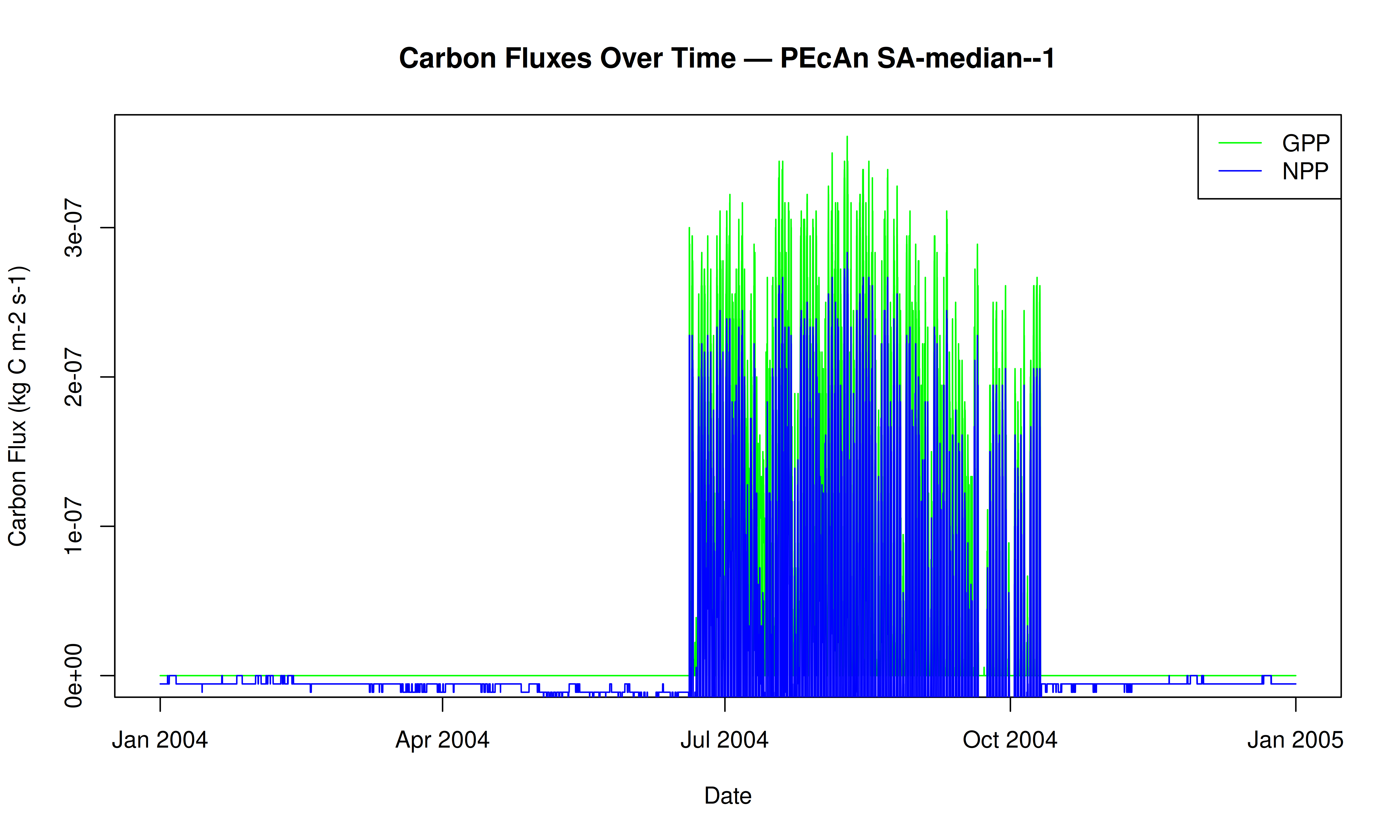
14.2 Plot Carbon Pools
# Plot Total Live Biomass and Total Soil Carbon
plot(model_output$posix, model_output$TotLivBiom,
  type = "l",
  col = "darkgreen",
  xlab = "Date",
  ylab = "Carbon Pool (kg C m-2)",
  main = paste("Carbon Pools Over Time — PEcAn", runid)
)
lines(model_output$posix, model_output$TotSoilCarb, col = "brown")
legend("topright", legend = c("Total Live Biomass", "Total Soil Carbon"), col = c("darkgreen", "brown"), lty = 1)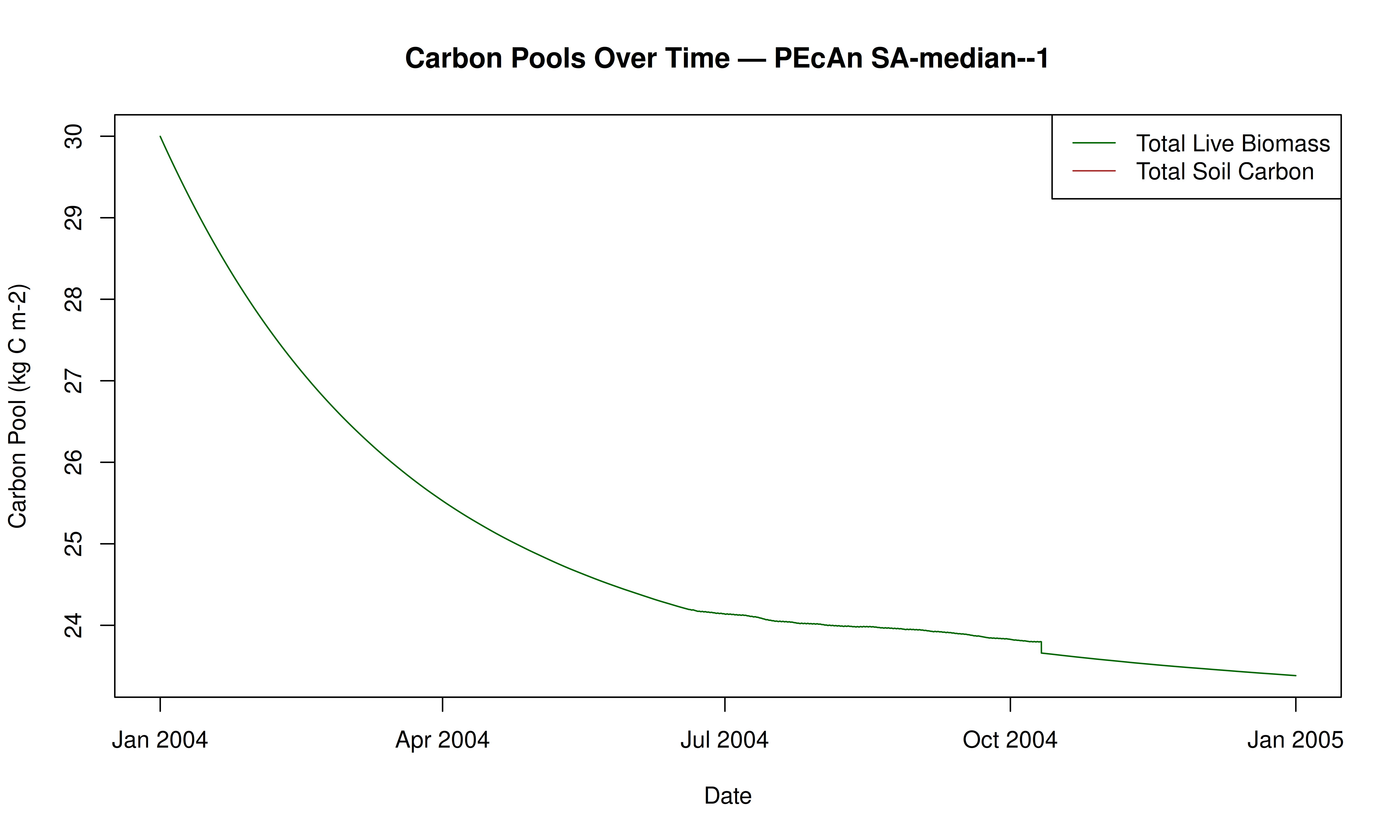
14.3 Plot Water Variables
# Plot Soil Moisture and Snow Water Equivalent
plot(model_output$posix, model_output$SoilMoist,
  type = "l",
  col = "blue",
  xlab = "Date",
  ylab = "Soil Moisture (kg m-2)",
  main = paste("Soil Moisture Over Time — PEcAn", runid)
)
lines(model_output$posix, model_output$SWE, col = "lightblue")
legend("topright", legend = c("Soil Moisture", "Snow Water Equivalent"), col = c("blue", "lightblue"), lty = 1)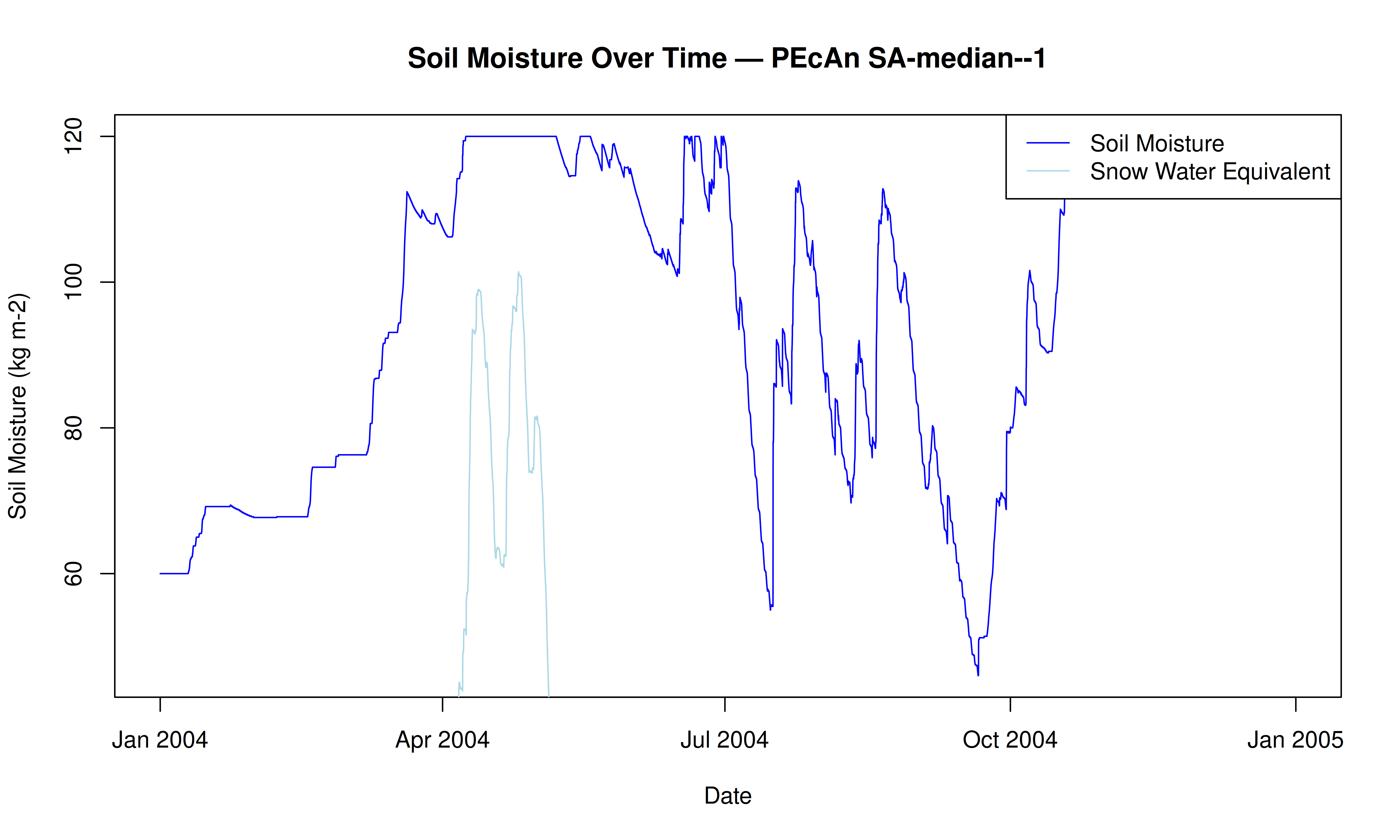
14.4 Plot LAI and Biomass
# Plot Leaf Area Index (LAI) and Above Ground Wood
plot(model_output$posix, model_output$LAI,
  type = "l",
  col = "darkgreen",
  xlab = "Date",
  ylab = "LAI (m2 m-2)",
  main = paste("Leaf Area Index Over Time — PEcAn", runid)
)
lines(model_output$posix, model_output$AbvGrndWood, col = "brown")
legend("topright", legend = c("LAI", "Above Ground Wood"), col = c("darkgreen", "brown"), lty = 1)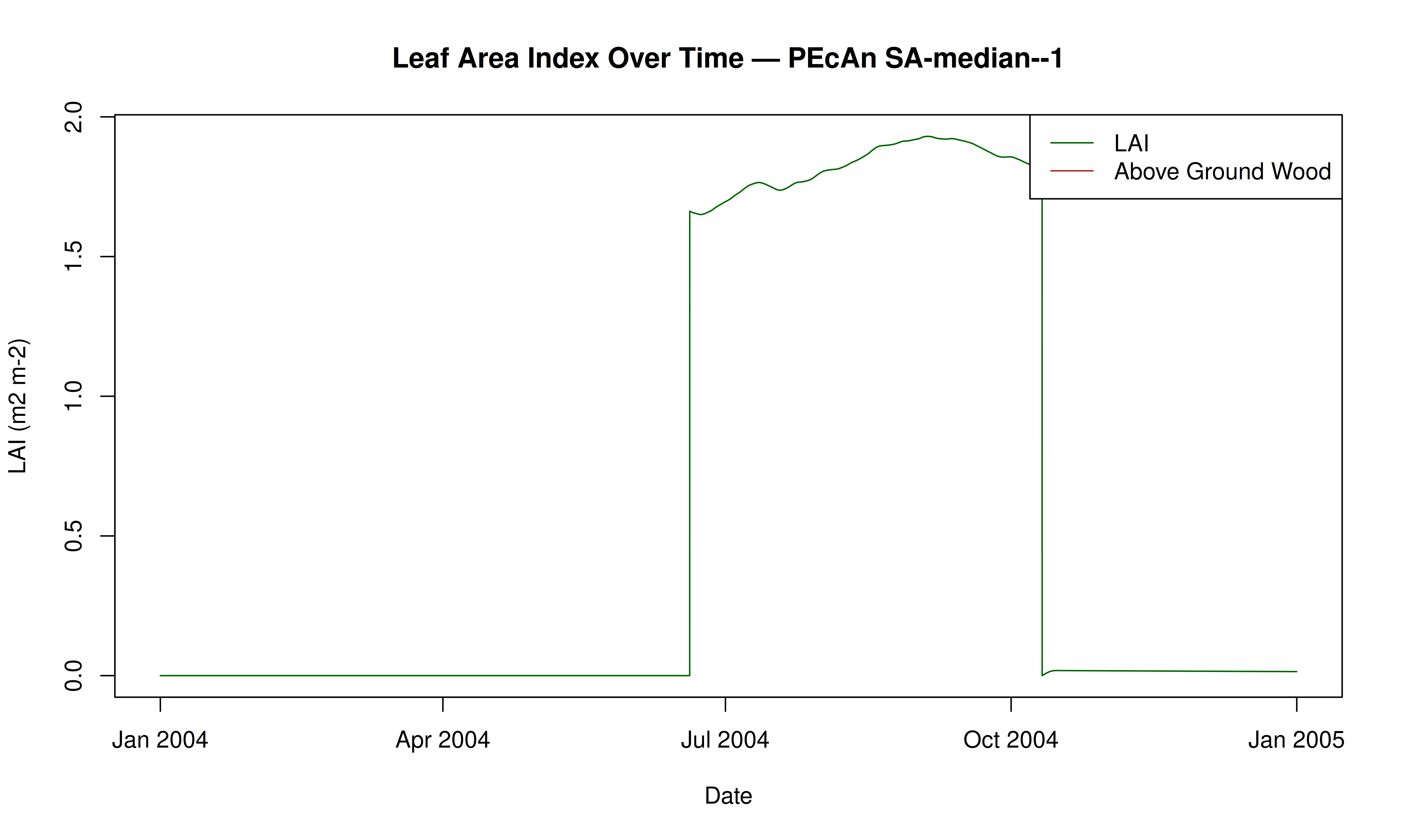
15 Conclusion
This notebook demonstrated how to set up, run, and analyze a PEcAn ecosystem model workflow programmatically. You can now modify parameters, try different models, or extend the analysis as needed.
Try editing the pecan.xml file. Give it a new name and update the settings_path variable at the beginning of this Demo to point to the new file. See how the changes affect the model output!
16 Further Exploration
The next set of tutorials will focus on the process of data assimilation and parameter estimation. The next two steps are in “.Rmd” files which can be viewed online.
Assimilation ‘by hand’
Explore how model error changes as a function of parameter value (i.e. data assimilation ‘by hand’)
MCMC Concepts Explore Bayesian MCMC concepts using the photosynthesis module
More info about tools, analyses, and specific tasks…
Additional information about specific tasks (adding sites, models, data; software updates; etc.) and analyses (e.g. data assimilation) can be found in the PEcAn documentation
If you encounter a problem with PEcAn that’s not covered in the documentation, or if PEcAn is missing functionality you need, please search known bugs and issues, submit a bug report, or ask a question in our chat room.
17 Clean Up Workflow Output (Optional)
If you want to remove all files and directories created by this workflow and start fresh, you can run the following code. This will delete the entire output directory specified in your settings. Use with caution!
# WARNING: This will permanently delete all workflow output files!
# Uncomment the line below to enable cleanup.
# fs::dir_delete(settings$outdir)
18 Session Information
18.0.1 PEcAn package versions.
PEcAn.all::pecan_version() package v1.10.0 installed source
PEcAn.all 1.10.0 1.10.0.9000 local (/pecan/bas...
PEcAn.allometry 1.7.5 1.7.5.9000 local (/pecan/mod...
PEcAn.assim.batch 1.9.1 1.9.1.9000 local (/pecan/mod...
PEcAn.BASGRA 1.8.2 1.8.2.9000 local (/pecan/mod...
PEcAn.benchmark 1.7.5 1.7.5.9000 local (/pecan/mod...
PEcAn.BIOCRO 1.7.5 1.7.5.9000 local (/pecan/mod...
PEcAn.CABLE 1.7.5 NA NA
PEcAn.CLM45 1.7.5 1.7.5.9000 local (/pecan/mod...
PEcAn.DALEC 1.7.5 1.7.5.9000 local (/pecan/mod...
PEcAn.data.atmosphere 1.9.1 1.9.1.9000 local (/pecan/mod...
PEcAn.data.land 1.9.0 1.9.0.9000 local (/pecan/mod...
PEcAn.data.mining 1.7.5 NA NA
PEcAn.data.remote 1.9.1 1.9.1.9000 local (/pecan/mod...
PEcAn.DB 1.8.2 1.8.2.9000 local (/pecan/bas...
PEcAn.dvmdostem 1.7.5 1.7.5.9000 local (/pecan/mod...
PEcAn.ED2 1.8.2 1.8.2.9000 local (/pecan/mod...
PEcAn.emulator 1.8.2 1.8.2.9000 local (/pecan/mod...
PEcAn.FATES 1.8.1 1.8.1.9000 local (/pecan/mod...
PEcAn.GDAY 1.7.5 1.7.5.9000 local (/pecan/mod...
PEcAn.JULES 1.7.5 1.7.5.9000 local (/pecan/mod...
PEcAn.LDNDC 1.0.2 1.0.2.9000 local (/pecan/mod...
PEcAn.LINKAGES 1.7.5 1.7.5.9000 local (/pecan/mod...
PEcAn.logger 1.8.4 1.8.4.9000 local (/pecan/bas...
PEcAn.LPJGUESS 1.9.0 1.9.0.9000 local (/pecan/mod...
PEcAn.MA 1.7.5 1.7.5.9000 local (/pecan/mod...
PEcAn.MAAT 1.7.5 1.7.5.9000 local (/pecan/mod...
PEcAn.MAESPA 1.7.5 1.7.5.9000 local (/pecan/mod...
PEcAn.ModelName 0.0.1 0.0.1.9000 local (/pecan/mod...
PEcAn.PEPRMT <NA> 0.1.0.9000 local (/pecan/mod...
PEcAn.photosynthesis 1.7.5 1.7.5.9000 local (/pecan/mod...
PEcAn.PRELES 1.7.5 NA NA
PEcAn.priors 1.7.5 1.7.5.9000 local (/pecan/mod...
PEcAn.qaqc 1.7.5 1.7.5.9000 local (/pecan/bas...
PEcAn.remote 1.9.1 1.9.1.9000 local (/pecan/bas...
PEcAn.RothC <NA> 0.0.0.9000 local (/pecan/mod...
PEcAn.settings 1.9.1 1.9.1.9000 local (/pecan/bas...
PEcAn.SIBCASA 0.0.3 0.0.3.9000 local (/pecan/mod...
PEcAn.SIPNET 1.10.0 1.10.9000 local (/pecan/mod...
PEcAn.STICS 1.8.2 1.8.2.9000 local (/pecan/mod...
PEcAn.uncertainty 1.9.0 1.9.0.9000 local (/pecan/mod...
PEcAn.utils 1.8.2 1.8.2.9000 local (/pecan/bas...
PEcAn.visualization 1.8.2 1.8.2.9000 local (/pecan/bas...
PEcAn.workflow 1.10.0 1.10.0.9000 local (/pecan/bas...
PEcAnAssimSequential 1.10.0 1.10.0.9000 local (/pecan/mod...
PEcAnRTM 1.9.1 1.9.1.9000 local (/pecan/mod...18.0.2 R session information:
sessionInfo()R version 4.4.3 (2025-02-28)
Platform: x86_64-pc-linux-gnu
Running under: Ubuntu 24.04.3 LTS
Matrix products: default
BLAS: /usr/lib/x86_64-linux-gnu/openblas-pthread/libblas.so.3
LAPACK: /usr/lib/x86_64-linux-gnu/openblas-pthread/libopenblasp-r0.3.26.so; LAPACK version 3.12.0
locale:
[1] LC_CTYPE=en_US.UTF-8 LC_NUMERIC=C
[3] LC_TIME=en_US.UTF-8 LC_COLLATE=en_US.UTF-8
[5] LC_MONETARY=en_US.UTF-8 LC_MESSAGES=en_US.UTF-8
[7] LC_PAPER=en_US.UTF-8 LC_NAME=C
[9] LC_ADDRESS=C LC_TELEPHONE=C
[11] LC_MEASUREMENT=en_US.UTF-8 LC_IDENTIFICATION=C
time zone: Etc/UTC
tzcode source: system (glibc)
attached base packages:
[1] stats graphics grDevices utils datasets methods base
other attached packages:
[1] PEcAn.SIPNET_1.10.9000 PEcAn.all_1.10.0.9000
[3] PEcAn.workflow_1.10.0.9000 PEcAn.remote_1.9.1.9000
[5] PEcAn.benchmark_1.7.5.9000 PEcAn.priors_1.7.5.9000
[7] PEcAn.emulator_1.8.2.9000 PEcAn.assim.batch_1.9.1.9000
[9] PEcAn.data.remote_1.9.1.9000 PEcAn.data.land_1.9.0.9000
[11] PEcAn.data.atmosphere_1.9.1.9000 PEcAn.uncertainty_1.9.0.9000
[13] PEcAn.utils_1.8.2.9000 PEcAn.logger_1.8.4.9000
[15] PEcAn.MA_1.7.5.9000 PEcAn.settings_1.9.1.9000
[17] PEcAn.DB_1.8.2.9000
loaded via a namespace (and not attached):
[1] PEcAn.qaqc_1.7.5.9000 DBI_1.2.3
[3] gridExtra_2.3 PEcAn.allometry_1.7.5.9000
[5] rlang_1.1.5 magrittr_2.0.3
[7] furrr_0.3.1 e1071_1.7-16
[9] compiler_4.4.3 vctrs_0.6.5
[11] stringr_1.5.1 pkgconfig_2.0.3
[13] PEcAn.MAESPA_1.7.5.9000 fastmap_1.2.0
[15] PEcAn.ED2_1.8.2.9000 labeling_0.4.3
[17] PEcAn.dvmdostem_1.7.5.9000 PEcAn.ModelName_0.0.1.9000
[19] rmarkdown_2.29 pracma_2.4.4
[21] sessioninfo_1.2.3 purrr_1.0.4
[23] xfun_0.52 PEcAn.JULES_1.7.5.9000
[25] jsonlite_2.0.0 PEcAn.LINKAGES_1.7.5.9000
[27] PEcAn.SIBCASA_0.0.3.9000 parallel_4.4.3
[29] R6_2.6.1 PEcAn.DALEC_1.7.5.9000
[31] stringi_1.8.7 PEcAn.CLM45_1.7.5.9000
[33] parallelly_1.43.0 numDeriv_2016.8-1.1
[35] lubridate_1.9.4 Rcpp_1.0.14
[37] iterators_1.0.14 knitr_1.50
[39] PEcAnAssimSequential_1.10.0.9000 igraph_2.1.4
[41] timechange_0.3.0 tidyselect_1.2.1
[43] abind_1.4-8 yaml_2.3.10
[45] PEcAn.LPJGUESS_1.9.0.9000 codetools_0.2-20
[47] listenv_0.9.1 lattice_0.22-6
[49] tibble_3.2.1 withr_3.0.2
[51] coda_0.19-4.1 evaluate_1.0.3
[53] future_1.34.0 sf_1.0-20
[55] units_0.8-7 proxy_0.4-27
[57] PEcAn.BASGRA_1.8.2.9000 pillar_1.10.2
[59] PEcAn.BIOCRO_1.7.5.9000 KernSmooth_2.23-26
[61] foreach_1.5.2 PEcAn.RothC_0.0.0.9000
[63] nimble_1.3.0 ncdf4_1.24
[65] generics_0.1.3 rprojroot_2.0.4
[67] ggplot2_3.5.2 munsell_0.5.1
[69] scales_1.3.0 globals_0.16.3
[71] PEcAn.MAAT_1.7.5.9000 PEcAn.STICS_1.8.2.9000
[73] class_7.3-23 glue_1.8.0
[75] tools_4.4.3 data.table_1.17.0
[77] XML_3.99-0.18 grid_4.4.3
[79] PEcAn.visualization_1.8.2.9000 tidyr_1.3.1
[81] PEcAn.photosynthesis_1.7.5.9000 colorspace_2.1-1
[83] PEcAn.PEPRMT_0.1.0.9000 cli_3.6.4
[85] PEcAnRTM_1.9.1.9000 dplyr_1.1.4
[87] PEcAn.GDAY_1.7.5.9000 gtable_0.3.6
[89] PEcAn.FATES_1.8.1.9000 digest_0.6.37
[91] classInt_0.4-11 PEcAn.LDNDC_1.0.2.9000
[93] rjson_0.2.23 htmlwidgets_1.6.4
[95] farver_2.1.2 htmltools_0.5.8.1
[97] lifecycle_1.0.4 here_1.0.1